Machine Learning free course – From Basics to Advanced

Hey there! So, you’re interested in diving into the fascinating world of machine learning (ML), huh? Awesome choice! Machine learning is one of the coolest and most powerful tools we have today. It’s changing the way we do just about everything, from recommending the next song you might like on Spotify to helping doctors diagnose diseases. But before we jump into the nitty-gritty, let’s get a good grasp of what machine learning is all about.

What is Machine Learning?

At its core, machine learning is a type of artificial intelligence (AI) that allows computers to learn from data and make decisions or predictions without being explicitly programmed to do so. Think of it like this: instead of writing a program that tells the computer exactly what steps to take, you create a model that learns from examples. The more data you feed it, the smarter it gets. Cool, right?

Supervised Learning

Let’s start with supervised learning, which is probably the most common type of machine learning. Imagine you’re teaching a child to recognize fruits. You show them pictures of apples and bananas and tell them which is which. Over time, they start to get the hang of it and can identify new apples and bananas on their own. That’s supervised learning in a nutshell.

In technical terms, supervised learning involves training a model on a labeled dataset. The model learns the mapping between input data (like images of fruits) and output labels (like “apple” or “banana”). Once trained, the model can predict the label for new, unseen data. Common algorithms used in supervised learning include linear regression, decision trees, and support vector machines (SVMs).

Unsupervised Learning

Next up, we have unsupervised learning. This one’s a bit different. Imagine you have a bunch of mixed-up Lego blocks, and you want to sort them without knowing what the final structures should look like. Unsupervised learning helps with this by finding patterns or groupings in the data.

In more technical terms, unsupervised learning deals with unlabeled data. The goal is to find hidden structures or relationships within the data. Clustering (like grouping customers with similar buying habits) and dimensionality reduction (like compressing high-dimensional data into simpler forms) are common tasks in unsupervised learning. Algorithms like k-means clustering and principal component analysis (PCA) are popular choices here.

The Machine Learning Pipeline

Okay, so now you know the basics of supervised and unsupervised learning. But how do we actually go from raw data to a working machine learning model? Enter the machine learning pipeline. This is a step-by-step process that includes:

1. Data Collection: Gathering the right data is crucial. Whether it’s from databases, sensors, or user inputs, the quality of your data will directly impact the performance of your model.
2. Data Cleaning: Raw data is often messy. This step involves handling missing values, removing duplicates, and correcting errors. Clean data is essential for building a reliable model.
3. Feature Engineering: This is where you select and transform the variables (features) that will be used by your model. Good features can make a huge difference in your model’s accuracy.
4. Model Training: Using the prepared data, you train your machine learning model. This involves selecting an algorithm and feeding it the data to learn from.
5. Model Evaluation: After training, you need to evaluate your model’s performance using metrics like accuracy, precision, recall, and F1 score. This helps you understand how well your model is doing.
6. Model Deployment: Once you’re satisfied with the model’s performance, it’s time to deploy it so it can start making predictions on new data.
7. Monitoring and Maintenance: The work doesn’t stop after deployment. You need to continuously monitor your model’s performance and update it as needed to ensure it remains accurate over time.

Common Applications of Machine Learning

Now that you have a handle on the basics, let’s talk about where machine learning is making waves:

1. Healthcare: From predicting disease outbreaks to personalizing treatment plans, machine learning is revolutionizing healthcare. For example, models can analyze medical images to detect early signs of conditions like cancer.
2. Finance: Banks and financial institutions use machine learning for fraud detection, credit scoring, and algorithmic trading. By analyzing transaction patterns, ML models can spot unusual activities that might indicate fraud.
3. Retail: Ever wondered how online stores know exactly what you might like to buy next? That’s machine learning at work, analyzing your browsing and purchase history to recommend products.
4. Entertainment: Streaming services like Netflix and Spotify use machine learning to suggest movies, shows, and songs based on your preferences. They analyze your past behavior to predict what you’ll enjoy next.
5. Autonomous Vehicles: Self-driving cars use a combination of supervised and unsupervised learning to navigate roads, avoid obstacles, and make driving decisions. They continuously learn from their environment to improve their performance.
6. Natural Language Processing (NLP): This is a branch of machine learning that focuses on the interaction between computers and human language. Applications include language translation, sentiment analysis, and chatbots.

Essential NumPy – Machine Learning

So, you’ve got a handle on the basics of machine learning. Now it’s time to roll up our sleeves and dive into some essential tools. One of the most fundamental libraries you’ll need to get familiar with is NumPy. Whether you’re just getting started with machine learning or venturing into the world of deep learning, NumPy is going to be your best friend. Trust me, mastering NumPy will make your life so much easier when working with data. Let’s break it down step by step.

Why NumPy?

NumPy (short for Numerical Python) is a powerful library for numerical computing in Python. It’s the backbone of many scientific computing applications and forms the foundation for other popular libraries like Pandas, TensorFlow, and scikit-learn. With NumPy, you can efficiently handle large arrays and matrices of numeric data, perform mathematical operations, and do a whole lot more.

Agenda

We’ll cover the following key topics to get you up and running with NumPy:

1. NumPy Creation: How to create arrays.
2. NumPy Access: Accessing elements in arrays.
3. NumPy hsplit, vsplit: Splitting arrays.
4. NumPy hstack, vstack: Stacking arrays.
5. NumPy Broadcasting: Efficiently performing operations on arrays of different shapes.

NumPy Creation

First things first, let’s talk about creating NumPy arrays. Arrays are the central data structure in NumPy. They are similar to Python lists but way more powerful. You can create arrays from lists or use functions like np.zeros, np.ones, np.arange, and np.linspace for more control.

Here’s a quick example:

import numpy as np
# Creating arrays from lists
arr1 = np.array([1, 2, 3, 4, 5])
arr2 = np.array([[1, 2, 3], [4, 5, 6]])
# Creating arrays using functions
arr_zeros = np.zeros((2, 3))  
# 2x3 array of zeros
arr_ones = np.ones((3, 2))    
# 3x2 array of ones
arr_range = np.arange(0, 10, 2)  
# Array with values from 0 to 10, step 2
arr_linspace = np.linspace(0, 1, 5)  
# 5 values evenly spaced between 0 and 1

NumPy Access

Accessing elements in NumPy arrays is pretty straightforward. You can use indexing and slicing just like with Python lists, but with more flexibility, especially for multi-dimensional arrays.

Check this out:

# 1D array
print(arr1[0])
  # First element
print(arr1[-1]) # Last element
# 2D array
print(arr2[0, 1])  
# Element in first row, second column
print(arr2[:, 1]) 
 # All elements in second column

NumPy hsplit, vsplit

Sometimes, you’ll need to split arrays into smaller sub-arrays. NumPy makes this easy with functions like hsplit (horizontal split) and vsplit (vertical split).

Here’s how it works:

# Splitting a 2D array horizontally
arr = np.array([[1, 2, 3, 4], [5, 6, 7, 8]])
hsplit_arr = np.hsplit(arr, 2)  
# Split into 2 sub-arrays
print(hsplit_arr)
# Splitting a 2D array vertically
vsplit_arr = np.vsplit(arr, 2) 
 # Split into 2 sub-arrays
print(vsplit_arr)

NumPy hstack, vstack

In contrast to splitting, you might need to stack arrays together. NumPy provides hstack (horizontal stack) and vstack (vertical stack) for this purpose.

Example time

arr3 = np.array([9, 10, 11, 12])
# Horizontal stacking
hstack_arr = np.hstack((arr, arr3.reshape(2, 2)))
print(hstack_arr)
# Vertical stacking
vstack_arr = np.vstack((arr, arr3.reshape(2, 2)))
print(vstack_arr)

NumPy Broadcasting

Broadcasting is one of NumPy’s most powerful features. It allows you to perform arithmetic operations on arrays of different shapes and sizes without explicitly reshaping them. This can save a lot of time and make your code cleaner.

Check out this magic:

arr4 = np.array([1, 2, 3])
arr5 = np.array([[0], [1], [2]])
# Broadcasting addition
broadcast_add = arr4 + arr5
print(broadcast_add)

We covered creating arrays, accessing elements, splitting and stacking arrays, and the powerful concept of broadcasting. Mastering these basics will set you up for success as you dive deeper into machine learning and data science.

Keep practicing and exploring more about NumPy. The more you use it, the more you’ll appreciate its power and flexibility. Stay curious and keep learning – you’re on the path to becoming a machine learning pro!

Essential NumPy – Machine Learning

Hey there! So, you’ve got a handle on the basics of machine learning. Now it’s time to roll up our sleeves and dive into some essential tools. One of the most fundamental libraries you’ll need to get familiar with is NumPy. Whether you’re just getting started with machine learning or venturing into the world of deep learning, NumPy is going to be your best friend. Trust me, mastering NumPy will make your life so much easier when working with data. Let’s break it down step by step.

Why NumPy?

NumPy (short for Numerical Python) is a powerful library for numerical computing in Python. It’s the backbone of many scientific computing applications and forms the foundation for other popular libraries like Pandas, TensorFlow, and scikit-learn. With NumPy, you can efficiently handle large arrays and matrices of numeric data, perform mathematical operations, and do a whole lot more.

Agenda

We’ll cover the following key topics to get you up and running with NumPy:

1. NumPy Creation: How to create arrays.
2. NumPy Access: Accessing elements in arrays.
3. NumPy hsplit, vsplit: Splitting arrays.
4. NumPy hstack, vstack: Stacking arrays.
5. NumPy Broadcasting: Efficiently performing operations on arrays of different shapes.

NumPy Creation

First things first, let’s talk about creating NumPy arrays. Arrays are the central data structure in NumPy. They are similar to Python lists but way more powerful. You can create arrays from lists or use functions like np.zeros, np.ones, np.arange, and np.linspace for more control.

Here’s a quick example:

import numpy as np
# Creating arrays from lists
arr1 = np.array([1, 2, 3, 4, 5])
arr2 = np.array([[1, 2, 3], [4, 5, 6]])
# Creating arrays using functions
arr_zeros = np.zeros((2, 3)) 
 # 2x3 array of zeros
arr_ones = np.ones((3, 2))    
# 3x2 array of ones
arr_range = np.arange(0, 10, 2)  
# Array with values from 0 to 10, step 2
arr_linspace = np.linspace(0, 1, 5) 
 # 5 values evenly spaced between 0 and 1<br>

NumPy Access

Accessing elements in NumPy arrays is pretty straightforward. You can use indexing and slicing just like with Python lists, but with more flexibility, especially for multi-dimensional arrays.

# 1D array
print(arr1[0]) 
 # First element
print(arr1[-1]) 
# Last element
# 2D array
print(arr2[0, 1])
  # Element in first row, second column
print(arr2[:, 1])  
# All elements in second column<br>

NumPy hsplit, vsplit

Sometimes, you’ll need to split arrays into smaller sub-arrays. NumPy makes this easy with functions like hsplit (horizontal split) and vsplit (vertical split).

# Splitting a 2D array horizontally
arr = np.array([[1, 2, 3, 4], [5, 6, 7, 8]])
hsplit_arr = np.hsplit(arr, 2)  
# Split into 2 sub-arrays
print(hsplit_arr)
# Splitting a 2D array vertically
vsplit_arr = np.vsplit(arr, 2) 
 # Split into 2 sub-arrays
print(vsplit_arr)<br>

NumPy hstack, vstack

In contrast to splitting, you might need to stack arrays together. NumPy provides hstack (horizontal stack) and vstack (vertical stack) for this purpose.

arr3 = np.array([9, 10, 11, 12])
# Horizontal stacking
hstack_arr = np.hstack((arr, arr3.reshape(2, 2)))
print(hstack_arr)
# Vertical stacking
vstack_arr = np.vstack((arr, arr3.reshape(2, 2)))
print(vstack_arr)

NumPy Broadcasting

Broadcasting is one of NumPy’s most powerful features. It allows you to perform arithmetic operations on arrays of different shapes and sizes without explicitly reshaping them. This can save a lot of time and make your code cleaner.

arr4 = np.array([1, 2, 3])<br>arr5 = np.array([[0], [1],[2]])
 # Broadcasting addition
 broadcast_add = arr4 + arr5
 print(broadcast_add)

Introduction to Pandas

Pandas is a powerful Python library for data analysis and manipulation. It provides two main data structures: Series and DataFrames. Think of Series as one-dimensional labeled arrays, and DataFrames as two-dimensional labeled arrays, sort of like spreadsheets or SQL tables. With Pandas, you can handle a wide variety of data formats, perform complex operations, and extract valuable insights from your data.

Understanding Series & DataFrames

Let’s start by getting familiar with Series and DataFrames. These are the building blocks of Pandas.

• Series: A Series is like a column in a table. It’s a one-dimensional array holding data of any type, along with an index that labels each element.

import pandas as pd
# Creating a Series
data = pd.Series([1, 3, 5, 7, 9])
print(data)<br>

DataFrames: A DataFrame is like a whole table. It’s a two-dimensional array with rows and columns, where each column can be of a different type.

# Creating a DataFrame
data = {   'Name': ['Alice', 'Bob', 'Charlie', 'David'],
'Age': [24, 27, 22, 32],
    'City': ['New York', 'Los Angeles', 'Chicago', 'Houston']}
df = pd.DataFrame(data)
print(df)

Loading CSV, JSON

One of the most common tasks you’ll encounter is loading data from files. Pandas makes this incredibly easy. Whether your data is in CSV, JSON, or other formats, Pandas has got you covered.

• Loading CSV files:

# Reading a CSV file
df_csv = pd.read_csv('path/to/your/file.csv')
print(df_csv.head())  
# Display the first few rows<br>

Loading JSON files:

# Reading a JSON file
df_json = pd.read_json('path/to/your/file.json')
print(df_json.head())

Connecting Databases

Need to pull data from a database? No problem. Pandas can easily connect to SQL databases using libraries like SQLAlchemy. This allows you to perform SQL queries and load the results directly into a DataFrame.

from sqlalchemy import create_engine

# Create a connection to the database
engine = create_engine('sqlite:///path/to/your/database.db')

# Execute a SQL query and load the data into a DataFrame
df_db = pd.read_sql_query('SELECT * FROM your_table', engine)
print(df_db.head())

Descriptive Statistics

Once you’ve got your data loaded, the next step is often to get a quick overview and some basic statistics. Pandas makes this super easy with its built-in functions.

• Basic statistics: You can use the describe method to get a summary of the central tendencies, dispersion, and shape of a dataset’s distribution.

# Get descriptive statistics
print(df.describe())

Other useful methods: Pandas provides a bunch of other handy methods to get specific statistics and insights.

print(df['Age'].mean())  # Mean of the Age column
print(df['Age'].median())  # Median of the Age column
print(df['Age'].value_counts())  # Frequency of unique values in the Age column

Accessing Subsets of Data – Rows, Columns, Filters

Alright, let’s dive deeper into how you can access and manipulate specific parts of your DataFrame. This is crucial for any data analysis or machine learning task.

• Accessing Rows: You can use loc and iloc to access rows. loc is label-based, while iloc is integer index-based.

# Accessing rows by index
print(df.loc[0])  # First row
print(df.iloc[2])  # Third row

Accessing Columns: Accessing columns is as simple as using the column name.

# Accessing columns
print(df['Name'])  # Access the 'Name' column

Filtering Data: You can filter your DataFrame based on conditions.

# Filtering data
print(df[df['Age'] > 25])  # Rows where Age is greater than 25

Handling Missing Data

Missing data is a common issue, and handling it properly is vital for accurate analysis.

• Identifying Missing Data: You can check for missing values using isnull and notnull.

# Identifying missing values
print(df.isnull())

Filling Missing Data: You can fill missing values with a specific value or a method (like forward fill).

# Filling missing values
df.fillna(0, inplace=True)  # Fill all NaNs with 0

Dropping Missing Data: Sometimes, it’s best to drop rows or columns with missing data.

# Dropping missing values
df.dropna(inplace=True)  # Drop rows with any NaN values

Dropping Rows & Columns

You might need to drop unnecessary rows or columns to clean your data.

• Dropping Rows: You can drop rows based on their index.

# Dropping rows
df.drop([0, 1], axis=0, inplace=True)  # Drop the first two rows

Dropping Columns: You can drop columns based on their names.

# Dropping columns
df.drop(['Age'], axis=1, inplace=True)  # Drop the 'Age' column

Handling Duplicates

Removing duplicate entries is essential for ensuring data quality.

• Identifying Duplicates: You can check for duplicate rows.

# Identifying duplicates
print(df.duplicated())

Dropping Duplicates: You can remove duplicate rows.

# Dropping duplicates
df.drop_duplicates(inplace=True)

Function Application – map, apply, groupby, rolling, str

Pandas provides powerful tools for applying functions across your data.

• map: Apply a function to each element in a Series.

# Using map
df['Age'] = df['Age'].map(lambda x: x + 1)  # Increment each age by 1

apply: Apply a function along any axis of the DataFrame.

# Using apply
df['Age'] = df['Age'].apply(lambda x: x * 2)  # Double each age

groupby: Group data by a column and apply aggregate functions.

# Using groupby
grouped = df.groupby('City').mean()  # Mean age by city
print(grouped)

rolling: Perform rolling window calculations.

# Using rolling
df['RollingMean'] = df['Age'].rolling(window=2).mean()  # Rolling mean with a window of 2

str: Apply string functions to Series containing strings.

# Using str
df['Name'] = df['Name'].str.upper()  # Convert names to uppercase

Merge, Join & Concatenate

Combining multiple DataFrames is a common task. Pandas makes it easy with merge, join, and concat.

• Merge: Similar to SQL joins.

# Using merge
df1 = pd.DataFrame({'key': ['A', 'B', 'C'], 'value': [1, 2, 3]})
df2 = pd.DataFrame({'key': ['A', 'B', 'D'], 'value': [4, 5, 6]})
merged = pd.merge(df1, df2, on='key', how='inner')  # Inner join on 'key'
print(merged)

Join: Join columns of another DataFrame.

# Using join
df1 = df1.set_index('key')
df2 = df2.set_index('key')
joined = df1.join(df2, lsuffix='_left', rsuffix='_right')
print(joined)

Concatenate: Stack DataFrames vertically or horizontally.

# Using concat
concatenated = pd.concat([df1, df2], axis=0)  # Concatenate along rows
print(concatenated)

Pivot-tables

Pivot tables are a powerful tool for summarizing data.

• Creating Pivot Tables: You can pivot your data to get a summarized view.

# Creating a pivot table
pivot_table = df.pivot_table(values='Age', index='City', aggfunc='mean')
print(pivot_table)

Normalizing JSON

Working with JSON data? Pandas can help you normalize and flatten nested JSON structures.

• Normalizing JSON: Convert nested JSON to a flat DataFrame.

import json

# Sample nested JSON
data = '{"Name": "Alice", "Details": {"Age": 24, "City": "New York"}}'

# Normalizing JSON
df_json = pd.json_normalize(json.loads(data))
print(df_json)

We’ve covered everything from accessing data subsets to handling missing data, dropping rows and columns, dealing with duplicates, applying functions, merging, joining, concatenating DataFrames, creating pivot tables, and normalizing JSON. With these skills in your toolkit, you’re well on your way to becoming proficient in data manipulation and analysis, setting a solid foundation for your machine learning projects. Keep exploring, experimenting, and learning – the data world is at your fingertips!

Linear Models for Regression & Classification 

Continuing with our journey into machine learning, let’s dive deeper into linear models for both regression and classification. This segment will cover various aspects, including the fundamental techniques, algorithms, and considerations for building effective models. Our agenda for this discussion includes:

1. Simple Linear Regression using Ordinary Least Squares (OLS)
2. Gradient Descent Algorithm
3. Regularized Regression Methods – Ridge, Lasso, ElasticNet
4. Logistic Regression for Classification
5. Online Learning Methods – Stochastic Gradient Descent & Passive Aggressive
6. Robust Regression – Dealing with outliers & Model errors
7. Polynomial Regression
8. Bias-Variance Tradeoff

Simple Linear Regression using Ordinary Least Squares (OLS)

Linear regression is the simplest and most commonly used predictive modeling technique. It assumes a linear relationship between the input variables (X) and the single output variable (y). Instead of diving into the mathematical formulas, let’s see how we can implement this using Python’s scikit-learn.

Code Implementation

import numpy as np
from sklearn.linear_model import LinearRegression
import matplotlib.pyplot as plt

# Sample data
X = np.array([[1], [2], [3], [4], [5]])
y = np.array([1, 3, 2, 5, 4])

# Create a linear regression model
model = LinearRegression()
model.fit(X, y)

# Make predictions
predictions = model.predict(X)

# Plot the results
plt.scatter(X, y, color='blue', label='Actual data')
plt.plot(X, predictions, color='red', linewidth=2, label='Linear regression line')
plt.legend()
plt.show()

Gradient Descent Algorithm

The Gradient Descent algorithm iteratively adjusts the model parameters to minimize the cost function. This approach is particularly useful for large-scale machine learning problems. Let’s implement a simple version of gradient descent.

Code Implementation

import numpy as np

# Sample data
X = np.array([1, 2, 3, 4, 5])
y = np.array([1, 3, 2, 5, 4])

# Parameters
learning_rate = 0.01
n_iterations = 1000
m = len(y)
theta_0 = 0
theta_1 = 0

# Gradient Descent Algorithm
for _ in range(n_iterations):
    y_pred = theta_0 + theta_1 * X
    d_theta_0 = -(2/m) * sum(y - y_pred)
    d_theta_1 = -(2/m) * sum((y - y_pred) * X)
    theta_0 = theta_0 - learning_rate * d_theta_0
    theta_1 = theta_1 - learning_rate * d_theta_1

print(f'Theta 0: {theta_0}, Theta 1: {theta_1}')

Regularized Regression Methods – Ridge, Lasso, ElasticNet

Regularization techniques help prevent overfitting by adding a penalty term to the cost function. We can easily implement these methods using scikit-learn.

Ridge Regression

from sklearn.linear_model import Ridge

# Create Ridge regression model
ridge = Ridge(alpha=1.0)
ridge.fit(X.reshape(-1, 1), y)
print("Ridge coefficients:", ridge.coef_)

# Make predictions
ridge_predictions = ridge.predict(X.reshape(-1, 1))

# Plot the results
plt.scatter(X, y, color='blue', label='Actual data')
plt.plot(X, ridge_predictions, color='green', linewidth=2, label='Ridge regression line')
plt.legend()
plt.show()

Lasso Regression

from sklearn.linear_model import Lasso

# Create Lasso regression model
lasso = Lasso(alpha=0.1)
lasso.fit(X.reshape(-1, 1), y)
print("Lasso coefficients:", lasso.coef_)

# Make predictions
lasso_predictions = lasso.predict(X.reshape(-1, 1))

# Plot the results
plt.scatter(X, y, color='blue', label='Actual data')
plt.plot(X, lasso_predictions, color='purple', linewidth=2, label='Lasso regression line')
plt.legend()
plt.show()

ElasticNet Regression

from sklearn.linear_model import ElasticNet

# Create ElasticNet regression model
elasticnet = ElasticNet(alpha=0.1, l1_ratio=0.5)
elasticnet.fit(X.reshape(-1, 1), y)
print("ElasticNet coefficients:", elasticnet.coef_)

# Make predictions
elasticnet_predictions = elasticnet.predict(X.reshape(-1, 1))

# Plot the results
plt.scatter(X, y, color='blue', label='Actual data')
plt.plot(X, elasticnet_predictions, color='orange', linewidth=2, label='ElasticNet regression line')
plt.legend()
plt.show()

Logistic Regression for Classification

Logistic Regression is used for binary classification problems. It models the probability that a given input belongs to a particular class. Let’s see how to implement logistic regression.

Code Implementation

from sklearn.linear_model import LogisticRegression

# Sample data
X = np.array([[0], [1], [2], [3], [4], [5]])
y = np.array([0, 0, 0, 1, 1, 1])

# Create a logistic regression model
model = LogisticRegression()
model.fit(X, y)

# Make predictions
predictions = model.predict(X)
print("Predictions:", predictions)

# Plot the results
plt.scatter(X, y, color='blue', label='Actual data')
plt.plot(X, model.predict_proba(X)[:, 1], color='red', linewidth=2, label='Logistic regression probability')
plt.legend()
plt.show()

Online Learning Methods – Stochastic Gradient Descent & Passive Aggressive

Online learning algorithms update the model incrementally as each new data point arrives. This is particularly useful for large datasets or streaming data.

Stochastic Gradient Descent (SGD)

from sklearn.linear_model import SGDRegressor

# Create SGD regression model
sgd = SGDRegressor(max_iter=1000, tol=1e-3)
sgd.fit(X.reshape(-1, 1), y)
print("SGD coefficients:", sgd.coef_)

# Make predictions
sgd_predictions = sgd.predict(X.reshape(-1, 1))

# Plot the results
plt.scatter(X, y, color='blue', label='Actual data')
plt.plot(X, sgd_predictions, color='brown', linewidth=2, label='SGD regression line')
plt.legend()
plt.show()

Passive Aggressive

from sklearn.linear_model import PassiveAggressiveRegressor

# Create Passive Aggressive regression model
pa = PassiveAggressiveRegressor(max_iter=1000, tol=1e-3)
pa.fit(X.reshape(-1, 1), y)
print("Passive Aggressive coefficients:", pa.coef_)

# Make predictions
pa_predictions = pa.predict(X.reshape(-1, 1))

# Plot the results
plt.scatter(X, y, color='blue', label='Actual data')
plt.plot(X, pa_predictions, color='cyan', linewidth=2, label='Passive Aggressive regression line')
plt.legend()
plt.show()

Robust Regression – Dealing with outliers & Model errors

Robust regression techniques are designed to be less sensitive to outliers and model errors. Methods such as RANSAC and Theil-Sen estimator are commonly used.

RANSAC Regression

from sklearn.linear_model import RANSACRegressor

# Create RANSAC regression model
ransac = RANSACRegressor()
ransac.fit(X.reshape(-1, 1), y)
print("RANSAC coefficients:", ransac.estimator_.coef_)

# Make predictions
ransac_predictions = ransac.predict(X.reshape(-1, 1))

# Plot the results
plt.scatter(X, y, color='blue', label='Actual data')
plt.plot(X, ransac_predictions, color='magenta', linewidth=2, label='RANSAC regression line')
plt.legend()
plt.show()

Theil-Sen Regression

from sklearn.linear_model import TheilSenRegressor

# Create Theil-Sen regression model
theil_sen = TheilSenRegressor()
theil_sen.fit(X.reshape(-1, 1), y)
print("Theil-Sen coefficients:", theil_sen.coef_)

# Make predictions
theil_sen_predictions = theil_sen.predict(X.reshape(-1, 1))

# Plot the results
plt.scatter(X, y, color='blue', label='Actual data')
plt.plot(X, theil_sen_predictions, color='gold', linewidth=2, label='Theil-Sen regression line')
plt.legend()
plt.show()

Polynomial Regression

Polynomial regression extends linear regression by adding polynomial terms of the input variables. This allows the model to fit non-linear relationships.

Code Implementation

from sklearn.preprocessing import PolynomialFeatures
from sklearn.linear_model import LinearRegression

# Sample data
X_poly = np.array([1, 2, 3, 4, 5]).reshape(-1, 1)
y_poly = np.array([1, 3, 2, 5, 4])

# Generate polynomial features
poly = PolynomialFeatures(degree=2)
X_poly_transformed = poly.fit_transform(X_poly)

# Create and fit the polynomial regression model
model_poly = LinearRegression()
model_poly.fit(X_poly_transformed, y_poly)

# Make predictions
poly_predictions = model_poly.predict(X_poly_transformed)

# Plot the results
plt.scatter(X_poly, y_poly, color='blue', label='Actual data')
plt.plot(X_poly, poly_predictions, color='red', linewidth=2, label='Polynomial regression line')
plt.legend()
plt.show()

Bias-Variance Tradeoff

The bias-variance tradeoff is a fundamental concept in machine learning. It describes the tradeoff between the error due to bias (error from erroneous assumptions in the model) and the error due to variance (error from sensitivity to small fluctuations in the training set).

Explanation with Example

To illustrate the bias-variance tradeoff, consider a scenario where we train a model with different levels of complexity:

In the above code, we train polynomial models of degrees 1, 3, and 9 and plot their fits along with training and testing data points. The train and test errors are printed to observe how increasing model complexity impacts bias and variance.

Linear models form the foundation of many machine learning algorithms. Understanding and mastering these techniques is essential for building robust and scalable models. By focusing on the code implementations and practical examples, you can gain a deeper insight into how these models work and how to apply them to real-world data.

Pre-Processing Techniques using Scikit-learn

Pre-processing is a crucial step in the machine learning pipeline. It involves transforming raw data into a format that can be easily and effectively used by machine learning models. Proper pre-processing can significantly improve the performance and accuracy of your models. In this section, we will discuss various pre-processing techniques using scikit-learn.

Introduction to Preprocessing

Preprocessing involves a series of steps to clean and transform data before feeding it into a machine learning model. The goal is to ensure that the data is in a suitable format for modeling and that it meets the assumptions of the algorithms being used. Some common preprocessing steps include scaling, normalization, binarization, encoding categorical features, imputation of missing values, and feature extraction.

Scikit-learn provides a robust set of tools for preprocessing data. These tools are implemented as transformers, which can be easily integrated into a machine learning pipeline.

StandardScaler

StandardScaler standardizes features by removing the mean and scaling to unit variance. This is particularly useful when the features in your dataset have different scales but similar ranges.

Explanation

StandardScaler works by computing the mean and standard deviation for each feature in the training data. It then scales the data to have zero mean and unit variance. This ensures that each feature contributes equally to the model, which is important for algorithms that are sensitive to the scale of the data, such as Support Vector Machines (SVM) and Principal Component Analysis (PCA).

from sklearn.preprocessing import StandardScaler
import numpy as np

# Sample data
data = np.array([[1, 2], [3, 4], [5, 6], [7, 8], [9, 10]])

# Initialize the StandardScaler
scaler = StandardScaler()

# Fit and transform the data
scaled_data = scaler.fit_transform(data)

print("Original Data:\n", data)
print("Scaled Data:\n", scaled_data)

Benefits and Use Cases

• Benefits: Standardizing data helps in improving the convergence speed of gradient-based algorithms. It also ensures that each feature contributes equally to the model.
• Use Cases: Useful in algorithms like SVM, PCA, and linear regression.

MinMaxScaler

MinMaxScaler scales and translates each feature individually such that it is in the given range, typically between zero and one.

Explanation

MinMaxScaler transforms features by scaling each feature to a given range. The default range is between zero and one, but it can be customized. This scaling is done by computing the minimum and maximum value of each feature and then transforming the data as follows:

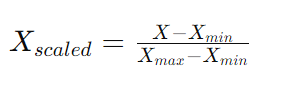
This technique is useful when you need to preserve the relationships between the data points while ensuring that the features are within a specific range.

from sklearn.preprocessing import MinMaxScaler

# Initialize the MinMaxScaler
min_max_scaler = MinMaxScaler()

# Fit and transform the data
min_max_scaled_data = min_max_scaler.fit_transform(data)

print("Original Data:\n", data)
print("Min-Max Scaled Data:\n", min_max_scaled_data)

Benefits and Use Cases

• Benefits: MinMaxScaler preserves the relationships between the data points and scales the data to a specific range, which can be useful for algorithms that require a bounded input space.
• Use Cases: Commonly used in neural networks, K-nearest neighbors (KNN), and any algorithm that requires feature scaling.

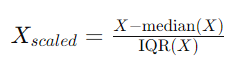
RobustScaler

RobustScaler uses statistics that are robust to outliers to scale the data. It removes the median and scales the data according to the interquartile range (IQR).

Explanation

RobustScaler is useful when your data contains outliers. Unlike StandardScaler, which uses mean and standard deviation, RobustScaler uses the median and IQR, making it more robust to outliers. The transformation is done as follows:

from sklearn.preprocessing import RobustScaler

# Initialize the RobustScaler
robust_scaler = RobustScaler()

# Fit and transform the data
robust_scaled_data = robust_scaler.fit_transform(data)

print("Original Data:\n", data)
print("Robust Scaled Data:\n", robust_scaled_data)

Benefits and Use Cases

• Benefits: RobustScaler is particularly useful when dealing with data that contains outliers, as it uses statistics that are less sensitive to outliers.
• Use Cases: Useful in scenarios where data has many outliers or skewed distributions.

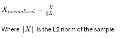
Normalization

Normalization scales individual samples to have unit norm. This is commonly used when working with machine learning models that require normalized inputs.

Explanation

Normalization adjusts the values of individual samples to ensure that they have a unit norm, which is calculated using the L2 norm (Euclidean norm). The transformation is done as follows:

from sklearn.preprocessing import Normalizer

# Initialize the Normalizer
normalizer = Normalizer()

# Fit and transform the data
normalized_data = normalizer.fit_transform(data)

print("Original Data:\n", data)
print("Normalized Data:\n", normalized_data)

Binarization

Binarization is a preprocessing technique that converts numerical features into binary values based on a specified threshold. This means that all values above the threshold are set to 1, and all values below or equal to the threshold are set to 0. Binarization is useful in feature engineering, particularly when dealing with algorithms that work well with binary features, such as logistic regression.

Explanation

Binarization transforms continuous numerical data into binary data. For instance, if you have a dataset with temperature readings, you might want to create a binary feature that indicates whether the temperature is above or below a certain threshold, such as freezing point. This can help highlight the presence or absence of certain conditions.

Code Implementation

Here’s how to implement binarization using scikit-learn:

from sklearn.preprocessing import Binarizer
import numpy as np

# Sample data
data = np.array([[1, 2], [3, 4], [5, 6], [7, 8], [9, 10]])

# Initialize the Binarizer with a threshold of 5
binarizer = Binarizer(threshold=5)

# Fit and transform the data
binarized_data = binarizer.fit_transform(data)

print("Original Data:\n", data)
print("Binarized Data:\n", binarized_data)

Benefits and Use Cases

• Benefits: Binarization helps in creating binary features from continuous data, which can simplify the data for certain models.
• Use Cases: Useful in scenarios where binary classification is required, such as detecting whether a temperature is above or below freezing point.

Encoding Categorical (Ordinal & Nominal) Features

Categorical data often needs to be converted into numerical format for machine learning models. There are two main types of categorical data: ordinal (with a meaningful order) and nominal (without a meaningful order). Encoding these features properly is crucial for model performance.

Explanation

1. Ordinal Encoding: Ordinal features have a meaningful order but no fixed interval between them. For example, ratings like “poor”, “average”, “good” can be encoded as 1, 2, 3.
2. One-Hot Encoding: Nominal features have no meaningful order. For example, color categories like “red”, “green”, “blue” should be encoded without implying any order. One-Hot Encoding creates binary columns for each category.

Ordinal Encoding

from sklearn.preprocessing import OrdinalEncoder

# Sample data
data = np.array([['low'], ['medium'], ['high'], ['medium'], ['low']])

# Initialize the OrdinalEncoder
ordinal_encoder = OrdinalEncoder(categories=[['low', 'medium', 'high']])

# Fit and transform the data
ordinal_encoded_data = ordinal_encoder.fit_transform(data)

print("Original Data:\n", data)
print("Ordinal Encoded Data:\n", ordinal_encoded_data)

One-Hot Encoding

from sklearn.preprocessing import OneHotEncoder

# Sample data
data = np.array([['red'], ['green'], ['blue'], ['green'], ['red']])

# Initialize the OneHotEncoder
one_hot_encoder = OneHotEncoder(sparse=False)

# Fit and transform the data
one_hot_encoded_data = one_hot_encoder.fit_transform(data)

print("Original Data:\n", data)
print("One-Hot Encoded Data:\n", one_hot_encoded_data)

Benefits and Use Cases

• Benefits: Proper encoding allows machine learning algorithms to process categorical data effectively.
• Use Cases: Useful in any scenario where categorical data is involved, such as demographic data, survey responses, etc.

Imputation

Imputation is the process of replacing missing values in a dataset. Handling missing values properly is essential because many machine learning algorithms cannot handle them directly.

Explanation

Imputation can be done in various ways, including:

1. Mean/Median Imputation: Replacing missing values with the mean or median of the column.
2. Most Frequent Imputation: Replacing missing values with the most frequent value in the column.
3. Constant Imputation: Replacing missing values with a constant value, such as 0 or ‘missing’.

Code Implementation

Mean/Median Imputation

from sklearn.impute import SimpleImputer
import numpy as np

# Sample data with missing values
data = np.array([[1, 2], [3, np.nan], [7, 6], [np.nan, 8], [9, 10]])

# Initialize the SimpleImputer for mean imputation
mean_imputer = SimpleImputer(strategy='mean')

# Fit and transform the data
mean_imputed_data = mean_imputer.fit_transform(data)

print("Original Data:\n", data)
print("Mean Imputed Data:\n", mean_imputed_data)

Most Frequent Imputation

# Initialize the SimpleImputer for most frequent imputation
freq_imputer = SimpleImputer(strategy='most_frequent')

# Fit and transform the data
freq_imputed_data = freq_imputer.fit_transform(data)

print("Most Frequent Imputed Data:\n", freq_imputed_data)

Benefits and Use Cases

• Benefits: Imputation helps in dealing with missing data without losing valuable information.
• Use Cases: Useful in any dataset with missing values, such as medical records, survey data, etc.

Polynomial Features

Polynomial features allow you to create new features by raising existing features to a power. This can help capture non-linear relationships in the data.

Explanation

Polynomial features transform the input features into polynomial terms, such as squares or cubes of the original features. This can help linear models capture non-linear relationships.

Code Implementation

from sklearn.preprocessing import PolynomialFeatures

# Sample data
data = np.array([[1, 2], [3, 4], [5, 6], [7, 8], [9, 10]])

# Initialize PolynomialFeatures with degree 2
poly = PolynomialFeatures(degree=2)

# Fit and transform the data
poly_features = poly.fit_transform(data)

print("Original Data:\n", data)
print("Polynomial Features Data:\n", poly_features)

Benefits and Use Cases

• Benefits: Polynomial features can help improve the performance of linear models by capturing non-linear relationships.
• Use Cases: Useful in regression tasks where the relationship between features and target is non-linear.

Custom Transformer

Custom transformers allow you to create your own preprocessing steps tailored to your specific needs. This is useful when you need to apply custom transformations that are not covered by standard preprocessing techniques.

Explanation

Custom transformers can be created by subclassing TransformerMixin and BaseEstimator from scikit-learn. This allows you to integrate your custom transformations into a scikit-learn pipeline.

Code Implementation

from sklearn.base import BaseEstimator, TransformerMixin
import numpy as np

class CustomTransformer(BaseEstimator, TransformerMixin):
    def fit(self, X, y=None):
        # Fit method, you can compute any statistics you need here
        return self

    def transform(self, X):
        # Transform method, apply your custom transformation here
        return np.log1p(X)

# Sample data
data = np.array([[1, 2], [3, 4], [5, 6], [7, 8], [9, 10]])

# Initialize and apply the custom transformer
custom_transformer = CustomTransformer()
transformed_data = custom_transformer.fit_transform(data)

print("Original Data:\n", data)
print("Transformed Data:\n", transformed_data)

Benefits and Use Cases

• Benefits: Custom transformers provide flexibility to apply specific transformations that are not available in standard preprocessing methods.
• Use Cases: Useful when you need to preprocess data in a unique way, such as applying domain-specific transformations.

Text Processing

Text processing is a critical step in natural language processing (NLP) and involves transforming raw text data into a format that can be used by machine learning models. This process includes tokenization, removing stop words, stemming, and lemmatization.

Explanation

1. Tokenization: Splitting text into individual words or tokens.
2. Stop Words Removal: Removing common words that do not contribute much to the meaning of the text (e.g., “and”, “the”).
3. Stemming: Reducing words to their base or root form (e.g., “running” to “run”).
4. Lemmatization: Similar to stemming but more accurate, reducing words to their base form based on dictionary definitions.

from sklearn.feature_extraction.text import CountVectorizer
import nltk
from nltk.corpus import stopwords
from nltk.stem import PorterStemmer, WordNetLemmatizer

# Sample text data
text_data = ["Natural language processing is fascinating.", 
             "Machine learning can be used to process natural language."]

# Tokenization and stop words removal
vectorizer = CountVectorizer(stop_words='english')
X = vectorizer.fit_transform(text_data)
print("Tokenized and Stop Words Removed:\n", X.toarray())

# Stemming
stemmer = PorterStemmer()
text_data_stemmed = [" ".join([stemmer.stem(word) for word in text.split()]) for text in text_data]
print("Stemmed Text:\n", text_data_stemmed)

# Lemmatization
lemmatizer = WordNetLemmatizer()
text_data_lemmatized = [" ".join([lemmatizer.lemmatize(word) for word in text.split()]) for text in text_data]
print("Lemmatized Text:\n", text_data_lemmatized)

Benefits and Use Cases

• Benefits: Text processing transforms unstructured text data into a structured format that can be used by machine learning models.
• Use Cases: Essential in NLP tasks such as sentiment analysis, topic modeling, and text classification.

CountVectorizer

CountVectorizer converts a collection of text documents to a matrix of token counts. This is a simple and commonly used text representation technique.

Explanation

CountVectorizer tokenizes the text and builds a vocabulary of known words. It then encodes the text documents as count vectors. Each row of the matrix represents a document, and each column represents a word from the vocabulary.

from sklearn.feature_extraction.text import CountVectorizer

# Sample text data
text_data = ["I love machine learning", "Machine learning is amazing"]

# Initialize CountVectorizer
vectorizer = CountVectorizer()

# Fit and transform the data
count_matrix = vectorizer.fit_transform(text_data)

print("Vocabulary:\n", vectorizer.vocabulary_)
print("Count Matrix:\n", count_matrix.toarray())

Benefits and Use Cases

• Benefits: Provides a simple way to convert text data into numerical format.
• Use Cases: Used in text classification, sentiment analysis, and topic modeling.

TfIdf (Term Frequency-Inverse Document Frequency)

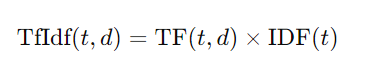
TfIdf is a statistical measure used to evaluate the importance of a word in a document relative to a collection of documents. It helps in identifying important words while reducing the weight of common words.

Explanation

TfIdf combines two metrics:

1. Term Frequency (TF): The number of times a word appears in a document.
2. Inverse Document Frequency (IDF): Measures the importance of a word by decreasing the weight of words that appear frequently in many documents.

The TfIdf value is calculated as:

from sklearn.feature_extraction.text import TfidfVectorizer

# Sample text data
text_data = ["I love machine learning", "Machine learning is amazing"]

# Initialize TfidfVectorizer
tfidf_vectorizer = TfidfVectorizer()

# Fit and transform the data
tfidf_matrix = tfidf_vectorizer.fit_transform(text_data)

print("Vocabulary:\n", tfidf_vectorizer.vocabulary_)
print("TfIdf Matrix:\n", tfidf_matrix.toarray())

Benefits and Use Cases

• Benefits: Helps in emphasizing important words while reducing the weight of common words, improving the performance of text classification models.
• Use Cases: Widely used in text classification, information retrieval, and text mining.

HashingVectorizer

HashingVectorizer is an alternative to CountVectorizer and TfidfVectorizer. It uses the hashing trick to convert text data into a fixed-dimensional vector.

Explanation

HashingVectorizer applies a hash function to the tokens to convert them into feature indices. This approach is faster and more memory-efficient since it does not require storing the vocabulary.

from sklearn.feature_extraction.text import HashingVectorizer

# Sample text data
text_data = ["I love machine learning", "Machine learning is amazing"]

# Initialize HashingVectorizer
hash_vectorizer = HashingVectorizer(n_features=10)

# Fit and transform the data
hash_matrix = hash_vectorizer.fit_transform(text_data)

print("Hash Matrix:\n", hash_matrix.toarray())

Benefits and Use Cases

• Benefits: More efficient in terms of memory usage and faster to compute, especially useful for large datasets.
• Use Cases: Suitable for high-dimensional text data and online learning scenarios.

Image Processing using skimage

Image processing involves manipulating and analyzing images to extract useful information. The skimage library in Python provides various functionalities for image processing, including transformations, filters, and feature extraction.

Explanation

Image processing steps may include resizing, normalization, edge detection, and more. These steps help in preparing the image data for machine learning models.

from skimage import io, color, filters
import matplotlib.pyplot as plt

# Load an example image
image = io.imread('https://example.com/path/to/image.jpg')

# Convert the image to grayscale
gray_image = color.rgb2gray(image)

# Apply a Gaussian filter
filtered_image = filters.gaussian(gray_image, sigma=1)

# Display the images
fig, ax = plt.subplots(1, 3, figsize=(15, 5))
ax[0].imshow(image)
ax[0].set_title('Original Image')
ax[1].imshow(gray_image, cmap='gray')
ax[1].set_title('Grayscale Image')
ax[2].imshow(filtered_image, cmap='gray')
ax[2].set_title('Filtered Image')
plt.show()

Benefits and Use Cases

• Benefits: Image processing helps in enhancing images, extracting features, and preparing image data for machine learning models.
• Use Cases: Widely used in computer vision tasks such as image classification, object detection, and image segmentation.

Decision Trees – Machine Learning

Decision Trees are a versatile machine learning algorithm that can be used for both classification and regression tasks. They are one of the simplest and most intuitive types of models, often used as the building blocks for more complex ensemble methods like Random Forests and Gradient Boosting Machines.

Introduction to Decision Trees

Decision Trees are tree-like models of decisions and their possible consequences, including chance event outcomes, resource costs, and utility. They are used to create a model that predicts the value of a target variable by learning simple decision rules inferred from the data features.

Key Concepts

1. Root Node: The topmost node in a decision tree, representing the entire dataset.
2. Decision Node: A node that splits into two or more sub-nodes.
3. Leaf/Terminal Node: A node that does not split further, representing a classification or decision.
4. Branch/Sub-Tree: A section of the entire tree.
5. Pruning: The process of removing sub-nodes to prevent overfitting.

Decision Trees can handle both numerical and categorical data. They work by recursively splitting the data into subsets based on the value of a chosen feature, creating branches until all the data is classified or a stopping condition is met.

The Decision Tree Algorithms

Several algorithms can be used to create decision trees. The most common ones are:

1. ID3 (Iterative Dichotomiser 3): Uses entropy and information gain to construct a decision tree.
2. C4.5: An extension of ID3 that handles both categorical and continuous data, and uses gain ratio instead of information gain.
3. CART (Classification and Regression Trees): Uses Gini impurity for classification and Mean Squared Error (MSE) for regression tasks.

Code Implementation

Here’s a basic implementation of a Decision Tree using scikit-learn’s CART algorithm:

from sklearn.datasets import load_iris
from sklearn.tree import DecisionTreeClassifier, plot_tree
import matplotlib.pyplot as plt

# Load dataset
iris = load_iris()
X, y = iris.data, iris.target

# Initialize and train the decision tree classifier
clf = DecisionTreeClassifier()
clf.fit(X, y)

# Plot the decision tree
plt.figure(figsize=(20,10))
plot_tree(clf, filled=True, feature_names=iris.feature_names, class_names=iris.target_names)
plt.show()

Decision Tree for Classification

Decision Trees are widely used for classification tasks. The algorithm splits the data based on the feature that results in the most homogeneous branches. This is typically measured using metrics such as Gini impurity or information gain (entropy).

Explanation

1. Gini Impurity: Measures the frequency at which any element of the dataset would be misclassified.
2. Entropy: Measures the amount of uncertainty or randomness in the data.

At each split, the algorithm chooses the feature that maximizes the reduction in impurity or increases the information gain.

from sklearn.model_selection import train_test_split
from sklearn.metrics import accuracy_score

# Split the data into training and test sets
X_train, X_test, y_train, y_test = train_test_split(X, y, test_size=0.3, random_state=42)

# Initialize and train the decision tree classifier
clf = DecisionTreeClassifier(criterion='gini')  # You can also use 'entropy'
clf.fit(X_train, y_train)

# Make predictions
y_pred = clf.predict(X_test)

# Evaluate the model
accuracy = accuracy_score(y_test, y_pred)
print(f"Accuracy: {accuracy * 100:.2f}%")

Decision Tree for Regression

For regression tasks, Decision Trees predict the target variable by learning decision rules from the features. Instead of using classification metrics like Gini impurity, regression trees use Mean Squared Error (MSE) to decide on splits.

Explanation

1. Mean Squared Error (MSE): Measures the average of the squares of the errors, i.e., the average squared difference between the estimated values and the actual value.

from sklearn.datasets import load_boston
from sklearn.tree import DecisionTreeRegressor
from sklearn.metrics import mean_squared_error

# Load dataset
boston = load_boston()
X, y = boston.data, boston.target

# Split the data into training and test sets
X_train, X_test, y_train, y_test = train_test_split(X, y, test_size=0.3, random_state=42)

# Initialize and train the decision tree regressor
regressor = DecisionTreeRegressor()
regressor.fit(X_train, y_train)

# Make predictions
y_pred = regressor.predict(X_test)

# Evaluate the model
mse = mean_squared_error(y_test, y_pred)
print(f"Mean Squared Error: {mse}")

dvantages & Limitations of Decision Trees

Advantages

1. Easy to Understand and Interpret: Decision Trees mimic human decision-making processes, making them easy to understand and visualize.
2. Requires Little Data Preprocessing: Decision Trees do not require feature scaling or centering.
3. Handles Both Numerical and Categorical Data: Decision Trees can work with a mix of feature types.
4. Non-Parametric: Decision Trees do not assume any underlying distribution for the data.

Limitations

1. Overfitting: Decision Trees can easily overfit the training data, especially if they are deep.
2. High Variance: Small changes in the data can result in a completely different tree.
3. Bias: Decision Trees tend to create biased trees if some classes dominate.
4. Computational Complexity: Finding the best split can be computationally intensive.

Mitigating Limitations

1. Pruning: Reduce the size of the tree by removing splits that have little importance.
2. Ensemble Methods: Techniques like Random Forests and Gradient Boosting combine multiple trees to reduce variance and improve performance.
3. Cross-Validation: Use cross-validation to tune the parameters of the tree and prevent overfitting.

Decision Trees are a powerful and intuitive tool in machine learning, offering clear advantages in terms of interpretability and ease of use. However, they also come with limitations that need to be managed through techniques like pruning, ensemble methods, and careful parameter tuning. Understanding both their strengths and weaknesses allows you to leverage Decision Trees effectively in various machine learning tasks.